---

Want some clever cell formatting in Excel but get confused by the Custom Format Cell options? Here is a quick tutorial to writing clever cell formats.

Getting started

Enter some data into your spreadsheet. To follow along with the tutorial step-by-step, enter the figures exactly as shown below, as this data has been specifically selected to illustrate how the custom formatting affects different types of values:

 

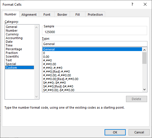
Select the cells, right-click on the range and click on Format Cells. Select the Custom category. You should see the following window:

By entering custom formatting codes into the “Type” field (where it says “General” in the above screenshot), you can affect the way your cell values display. These custom formatting codes are

broken into four sections, separated by semicolons, to specify how four different types of values will be represented:

Positive numbers; negative numbers; zeroes; text

Your first custom format

Let’s say you want to display a comma every third digit and force a negative sign to appear before any negative values.

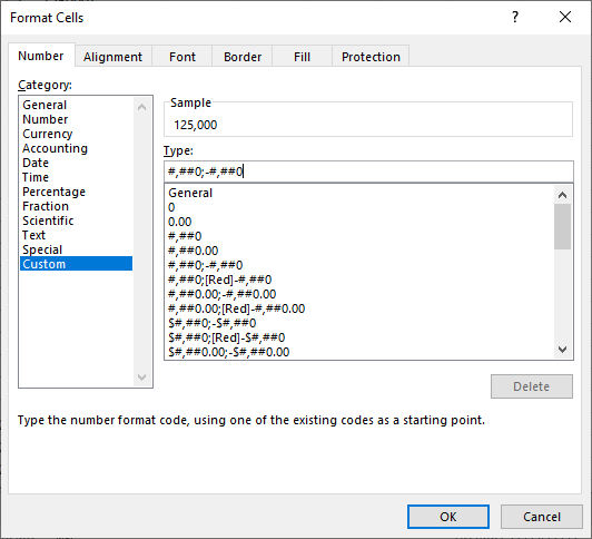
The custom format code: #,##0;-#,##0

Going from left to right, this code tells Excel how to format the positive numbers before the semicolon, then the negative numbers after the semicolon. Because there are no more semicolons or codes after that, the zeroes and text will display the same as “General” formatting.

To display the data you have entered in your custom format, paste the code above into the “Type” field as shown below:

Once you click “OK”, your formatted cells should look like this:

Let’s explore some more examples

The code: #,##0.00;-#,##0.00

What it does: Same as the previous examples, but with two decimals displayed after each value, including zeroes.

The formatted cells:

The code: #,##0;-#,##0;

What it does: Looks like the first example, but the extra semicolon on the end will make any cells containing an overall value of zero appear blank.

The formatted cells:

The code: #,##0;;

What it does: This will hide any negatives or zeros as no format has been given for their display. (Put another semicolon on the end, and all text entries will also be invisible #,##0;;; )

The formatted values:

Custom formats with dollar signs

The code: $#,##0;-$#,##0

What it does: Puts the $ next to the leftmost number.

The formatted cells:

The code: _-$* #,##0;-$* #,##0

What it does: Puts the $ on the left of the cell. The _- is to leave enough room to the left of the $ for the – sign on negative numbers. The * followed by a space before the # indicates filling the remainder of the cell with spaces.

The formatted cells:

Custom formats with special codes

The code: **;**;**;**

What it does: Will display * across all cells (as if hiding a password).

Example of formatted cells:

Custom formats with larger numbers

For these final examples, you’ll need to enter some larger numbers. In the screenshots below, you can see the numbers entered with “General” formatting on the left and the formatted cells on the right.

The code: 0.0,, “M”

What it does: Will display millions as smaller values.

The formatted values:

The code: $0.0,, “M”

What it does: Will also display the millions with $ sign.

The formatted values: