There is so much you can do with conditional formatting in Excel, and you will save yourself a lot of time in the long term if you take a little time to learn a few tricks. If you are new to conditional formatting, one quite easy feature to get you started is highlighting duplicated data.
Finding duplicate cells in a column
Step 1. Select a column containing possible duplicates.
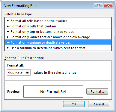
Step 2. Go to: Home > Conditional Formatting > New Rule > Format only unique or duplicate values
Step 3. Select duplicate from the format all dropdown list.

Step 4. Click Format and choose a colour to identify the duplicate cells, then click OK to select your choices.
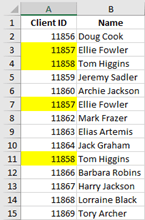
Step 5.Click OK again to apply the formatting rule. All duplicate rows are now highlighted.

Using format painter to copy conditional formatting and highlight duplicate rows
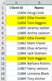
To extend your conditional formatting to highlight completely duplicated rows of data, rather than just duplicate cells within the same column, use Format Painter.
Step 1. Start by selecting the cells in the column that already has the conditional formatting rule applied.
Step 2. Click on Format Painter in the Home toolbar.
Step 3. Use the format painter, drag to select the cells from the other column or columns you would like to apply the conditional formatting to.

Filtering to display only duplicate cells
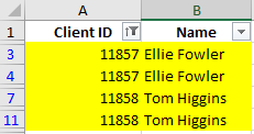
Step 1. Ensure your filter arrows are showing by going to Data > Filter.
Step 2. Select the filter arrow and choose Filter by Colour, choosing your colour.

Only the duplicate records will display. Sorting might also show the duplicates grouped together.

This tip was provided by Jane Pettigrew, one of our expert Microsoft trainers. Learn more by attending our beginner to advanced level Microsoft Excel training.


