1: Viewing multiple sheets of the same workbook

Have you ever wanted to see the content of two sheets of the same workbook side by side at once? From the View tab, click New Window. This opens another window, with the same file viewed again. Click Arrange All, choose Tiled, and the file will appear twice, side by side. Click on another sheet in the second window to view its contents.

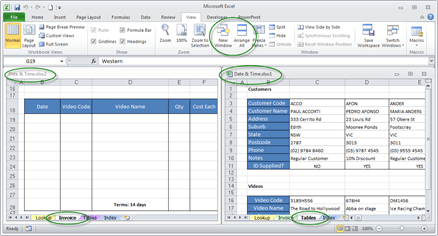
It’s important to note this isn’t a copy of the file, just another ‘view’. Changes made in one side of the screen are made in the other, too. To return to normal, simply close one of the windows, and maximise the screen again.

2: Make a message pop up when a cell is selected

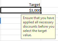
You could use a comment to add a message to a cell, but then you need to click on the comment marker to read the message. If you want to always display the message when the cell is selected, try using an Input Message. Select your cell, and from the Data tab of the ribbon, select Data Validation. Click on the Input Message tab, and type the message to appear. Click OK and the message will always pop up when the cell becomes active.

3: Centre cells across selection

Are you tired of getting error messages about merged cells? Merged cells can make your worksheet look good, but when you start to copy and paste, and the ghastly “Can’t copy part of a merged cell” message appears. There is a little used feature that lets you centre text across multiple cells, without actually merging them. But this feature only works when you want to merge across columns. There is no way to do this for merging down.

Type your heading in the leftmost cell. Select the range of cells you want to centre across. From the Home tab, Alignment group, click the dialog box launcher . Select the Horizontal alignment and choose – Center Across Selection.

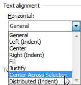
The text will look centred but all the other cells will need to remain blank for the illusion to remain.

4: Using outlines to hide content quickly

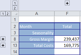
Are you always hiding/unhiding rows and columns for printing or displaying your content in presentations? Why not use an Outline instead? One click and you can easily hide or unhide specific content. Select the columns or rows to hide. From the Data tab on the ribbon, select Group. The outline appears across the top or down the side.

Click the outline buttons to show/hide rows or columns as you need them.

5. Quickly displaying formulas

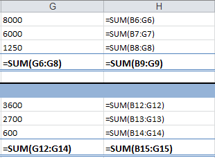
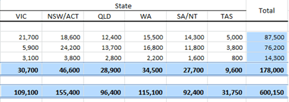
When confronted with a spreadsheet that you’ve not seen before, it can be daunting to locate all the cells containing formulas. Press the CTRL+` keys (HINT: the ` is to the left of the 1 on most keyboards). All cells containing formulas will display the formula in cell! Press it again to go back to normal. Use this to locate and view formulas, and even print them.

Ok, I lied, there is one more tip. What if you want to quickly select all the cells containing formulas? Simply press F5, then click Special, and choose Formulas. All cells containing formulas will be selected!

Finally…

There are dozens of ways to quickly get the results you want with Excel. Take some time to explore buttons on the ribbon you’ve never used before, or to learn what the keyboard shortcuts can do to save you time.

Enhance your computer training skills with courses at Odyssey Training.